Multifamily Opportunistic Pro Forma Model

About This Model

Why Opportunistic Underwriting Breaks Templates

The opportunistic multifamily acquisition is the deal that ate the spreadsheet. A standard value-add model assumes you take over a partially-occupied asset, push rents, hold for five years, and exit. An opportunistic deal isn't that. You are buying something that doesn't work yet (distressed occupancy, deferred maintenance, broken capital structure, or all three) and the work to make it work happens during the hold period, financed by debt that has to be retired or replaced before you can claim a stabilized valuation.

Three things have to be modeled at once, and they interact:

1. Physical repositioning. Phased renovation of unit interiors, exteriors, and amenities, on a construction-style draw schedule, with contingency. The capital is real-time, not amortized.
2. Financial repositioning. Bridge debt during the work, refinanced into permanent financing at stabilization. The bridge has an interest reserve, a rate cap, extension options, and a holdback that releases against operational milestones. The perm sizing is constrained by DSCR floors against stabilized NOI.
3. Operational repositioning. Lease-up from initial occupancy through stabilization, with market-rate concessions, turnover assumptions, and absorption curves that are nonlinear in shape.

A model that handles any two of the three on a single sheet will mis-size the third. The most common failure mode is treating renovation as a Year-1 capex line item. Capex in Year 1 spreads $4M of renovation evenly across twelve months. Real renovation programs draw in phases (exteriors in months 1–6, interiors as units turn in months 4–14, amenities in months 9–15) and peak monthly draws can be 4× the smoothed average. If you are sizing a bridge facility off the smoothed number, your interest reserve is wrong, your holdback release schedule is wrong, and the DSCR test at refinance is wrong.

The second-most-common failure is linear lease-up. A 200-unit asset starting at 70% occupancy that targets 95% in eighteen months will absorb roughly two units per month on a linear curve. Actual absorption rarely looks like that. Lease-up follows a logistic shape: slow at first while you reposition the brand and burn off prior tenants, accelerating through the middle period when marketing hits a stride, and tapering as you approach the stabilized occupancy ceiling. We will get to why that matters in the next section.

The third failure is the waterfall. Opportunistic deals are almost always structured with multi-tier promote schedules: return of capital, preferred return, catch-up, then two or three IRR-tested hurdle tiers. A simple promote can model a JV with one LP and one GP, but it cannot model the structures that opportunistic capital actually shows up in.

AQ-141 was engineered to handle all three at once on a model a single user can audit in a week. The rest of this piece is a tour of the choices we made.

Design Choice: S-Curve Absorption

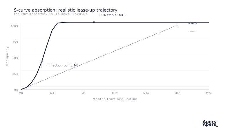
AQ-141 uses a logistic function to model lease-up absorption rather than a linear ramp or a fixed monthly leasing-velocity assumption. The decision sounds like a modeling preference. It is closer to a solvency decision.

The logistic function we implemented:

occupancy(t) = O₀ + (L - O₀) / (1 + e^(-k(t - m)))

Where O₀ is initial occupancy, L is target stabilized occupancy, k is the curve steepness, and m is the inflection month at which absorption velocity peaks. The user supplies initial occupancy, target occupancy, the ramp start month, the inflection month, and the steepness. The model computes per-month occupancy across up to 36 months of lease-up, then converts that into per-month effective gross income, operating expenses, and net operating income.

Why not linear

A linear ramp from 70% to 95% over eighteen months delivers 1.39 net absorbed units per month on a 200-unit asset. Steady, easy to model, easy to explain. The problem is that no real lease-up looks like that, and the deviation matters at exactly the wrong time.

Real absorption is back-loaded. The first three to six months of an opportunistic hold are dominated by repositioning: rebranding the asset, terminating problem leases, renovating model units, repointing exterior fixtures, and rebuilding the property-management infrastructure. New leases trickle in during this window because your sales staff is still selling against a half-renovated building. Months six through twelve are when the machine starts working (the model units are done, the website is up, the leasing office is staffed) and absorption velocity reaches its peak. Months twelve through eighteen taper as you approach stabilized occupancy and the marginal renter becomes harder to find.

A linear model overstates NOI in months 1–9 and understates it in months 10–18. Most of the time the misstatement is small enough that you don't notice. But the worst months, the early ones, when actual occupancy is below linear, are also the months when bridge interest coverage is tightest. If your interest reserve was sized off a linear ramp, you are short reserve in exactly the months you need it.

Why monthly, not annual

Lease-up risk is binary at the loan level. The bridge facility tests DSCR monthly (or quarterly, depending on documents) against operating cash flow. A month with a DSCR below the facility floor triggers a cash sweep, a holdback freeze, or, depending on documents, an event of default. Annual cash flow can look healthy while three individual months trip the test.

For this reason AQ-141 runs the lease-up period at monthly granularity for up to 36 months, then transitions to annual cash flow modeling for the remainder of the hold. The handoff is at the user-specified stabilization date, not at a fixed calendar year, because opportunistic deals stabilize on their own schedule.

What we made tunable

The four inputs to the absorption curve (O₀, L, k, m) were chosen because they correspond to actual underwriter intuition. Initial and target occupancy are obvious. Inflection month is the answer to "when does this thing start leasing?", which experienced operators have a strong view on. Steepness is the answer to "how fast does it absorb once it's working?", which is a function of the submarket's depth and the property's competitive position.

We deliberately did not expose seasonal-adjustment factors, weekly leasing velocity, traffic-to-lease conversion ratios, or rent concession schedules. Those are second-order effects relative to the absorption curve itself, and exposing them is the first step toward an unauditable model. A user who needs them is a user who should be in a bespoke model, not a template.

Design Choice: Phased Renovation with Construction-Style Draws

Renovation in AQ-141 is modeled as a construction project, not as a capex line item. The user enters per-unit renovation cost segmented by scope (light, medium, heavy) and the model produces a monthly draw schedule, tracks budgeted-versus-spent, applies contingency, and feeds the result into the bridge debt model.

The reason is that opportunistic capex doesn't behave like maintenance capex. A $4M renovation program across 200 units is a real construction operation with a critical path, sequencing constraints, and cash flow timing that has very little to do with the calendar.

Why per-scope, not per-unit

Each unit in the rent roll is tagged with a renovation scope (none, light, medium, or heavy) and the model applies a per-scope cost from the assumptions sheet rather than a per-unit cost. There are two reasons for this.

First, opportunistic underwriting almost never has unit-by-unit cost detail at deal stage. You have a walk-through note that says "60 units need a full gut, 80 need cabinets and counters, 60 are mostly cosmetic." Pretending you have unit-level cost precision implies a level of diligence that doesn't exist yet.

Second, the scope-level abstraction is durable. When the contractor's bid comes back and the "light" scope turns out to be $8,500 rather than $7,200, you change one cell. A unit-level cost model would force you to update sixty cells, which means you don't update it, which means the model drifts away from reality the moment the deal goes under contract.

Why monthly draws

The draw schedule is the bridge between the renovation plan and the bridge facility. Bridge lenders fund against monthly draws, hold a percentage as holdback, and release the holdback against stabilization milestones. If you are not modeling the draws monthly, you cannot size the facility, the interest reserve, or the holdback release schedule.

The model defaults to an S-curve draw shape that front-loads soft costs (design, permitting, mobilization) in months 1–3, ramps hard costs (interiors, mechanicals, exteriors) through the middle of the program, and tapers punch-list and final inspection items at the end. The shape is editable per scope so that exterior work, which typically front-loads, can have a different curve than interior unit renovations, which back-load behind unit turnover.

Why contingency is tracked, not buried

AQ-141 tracks contingency as a separate column in the renovation budget rather than rolling it into per-scope cost. A 10% contingency on a $4M program is $400K. If that money is buried inside the line-item cost, three things break: the lender's underwriting test against your "hard cost" budget is wrong; your IC presentation misstates the capital need; and when you eventually spend the contingency, you can't tell whether it was deployed against true cost overruns or scope creep.

The contingency line is reported in the sources-and-uses, drawn down as cost overruns are recognized, and tracked against the original budget. The model does not pretend to predict contingency utilization; it only ensures the column exists.

Design Choice: Bridge-to-Permanent Refinance Architecture

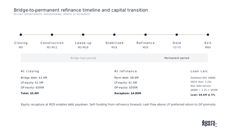
The single largest engineering decision in AQ-141 was how to model the transition from bridge debt to permanent financing. We chose to model it as a single, dated refinance event with explicit interest reserve testing, rate cap amortization, and holdback release mechanics.

The alternative (modeling continuous debt with a rate step at stabilization) is more flexible but harder to audit. Almost all opportunistic deals refinance exactly once, from a bridge facility (typically 3–5 years with 1–2 extensions) into agency or CMBS perm debt. Building the model to support multiple refinances would have forced complexity onto users whose deals do not need it.

How the refi mechanics work

The refinance event happens at a user-specified month and triggers four cash flow movements:

1. Permanent loan sizing. The new loan is sized off the trailing-twelve-month stabilized NOI against three constraints: LTV against stabilized valuation, DSCR floor against stabilized NOI at the perm rate, and a maximum loan amount. The binding constraint sets the proceeds.
2. Bridge payoff. Outstanding bridge principal, accrued interest, prepayment fees (if any), and unused interest reserve return are netted at refinance.
3. Holdback release. The bridge facility's holdback (typically 10–15% of the original commitment) is funded into the borrower at stabilization rather than at closing. AQ-141 models this as a positive cash flow to the deal at the refinance month, reducing the equity contribution required at closing.
4. Refinance proceeds. If the perm loan amount exceeds the bridge payoff, the excess flows back to the deal as a distributable refinance event. This is where opportunistic deals make a meaningful portion of their levered returns. The cash-out at refi often exceeds the cash-on-cash through the hold.

Why we model the holdback explicitly

Bridge facility holdbacks are the most under-modeled mechanic in opportunistic underwriting. A facility commits $50M, funds $42–45M at close, and releases the remaining $5–8M against stabilization milestones (a DSCR test, an occupancy threshold, or both). If you treat the facility as fully funded at close, you understate the equity requirement through the hold and overstate the cash-on-cash in the lease-up period.

AQ-141 takes the holdback percentage as a user input, ties its release to a user-defined stabilization condition, and reports the peak equity requirement net of holdback. The peak equity figure is what the GP actually has to raise, not the headline LTC.

Stress-testing extensions

Bridge facilities almost always carry two extensions of six to twelve months each, priced with a fee (typically 25–50 bps) and a rate step-up (typically 25–100 bps SOFR spread). Each extension is independently togglable in the model. The default base case assumes no extensions are exercised; the downside scenario engages both. This matters because the most common reason opportunistic deals miss returns is that lease-up takes longer than underwritten, the perm refi is delayed, and the GP eats two rounds of extension fees and step-up interest before refinancing into a worse rate environment.

Design Choice: Interest Reserve Sizing and Stress Testing

The interest reserve is the cushion of capital, set aside at closing, that pays bridge debt service when operating cash flow doesn't cover it. Sizing the reserve correctly is one of the deal-killing details in opportunistic underwriting. Too small, and the deal trips DSCR mid-renovation. Too large, and you are tying up LP capital that should be working.

AQ-141 sizes the reserve as a function of three inputs: months of expected lease-up shortfall, average expected shortfall per month, and a buffer. The model then runs a per-month test that compares operating cash flow plus reserve drawdown against debt service. A month in which the combined coverage falls below the facility's DSCR floor is flagged in the output as an interest reserve adequacy failure.

The decision: rule-of-thumb vs. computed

A common practice is to size the reserve at "12 months of debt service" as a rule of thumb. We rejected this framing. The right size is the cumulative shortfall between projected operating cash flow and required debt service across the lease-up period, plus a buffer. Twelve months of debt service might be too much (if NOI ramps fast and the deficit period is short) or far too little (if absorption is slow and the deficit period stretches eighteen months).

The model computes the cumulative shortfall directly from the lease-up cash flow projection and the bridge debt service schedule. The user adds a buffer percentage on top (we default to 20%) to absorb the gap between the base-case shortfall and a realistic downside.

Why we test against the facility floor, not against zero

A reserve that is "adequate" in the sense of "doesn't run out" is not adequate in the sense of "passes the facility's DSCR test." Most bridge facilities require a 1.05–1.15x DSCR even during lease-up, with cash sweeps triggered below the floor. The model's reserve adequacy test is run against the facility's actual covenant level, which the user inputs from the loan term sheet. A month that passes a zero-coverage test but fails the covenant-level test still triggers a sweep, and a sweep delays the holdback release, which delays the refi, which delays the return.

Design Choice: Waterfall Architecture

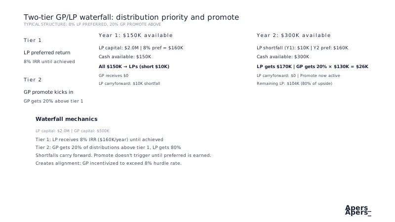
The distribution waterfall is the second-largest engineering decision in the model. AQ-141 supports two architectures via a single toggle: a simple promote with one pref tier and one carry tier, and a multi-tier IRR hurdle structure with up to three hurdle tiers, GP catch-up, and GP co-invest.

Why a toggle instead of two models

Most opportunistic GPs use the multi-tier structure with their institutional capital and the simple structure with their friends-and-family co-invest. Forcing them to maintain two separate models (one per structure) creates the worst of all worlds: two files to update, two files to audit, and a coin flip on which one is the "right" version for any given LP conversation.

The toggle in AQ-141 routes cash flow distributions through either the simple or the multi-tier engine based on a single cell. The output sheets (partner-level IRRs, equity multiples, cash-on-cash, GP promote earned) render identically regardless of which engine is active. The user is in one file, talking to one LP at a time, in the structure that LP cares about.

The multi-tier engine

The multi-tier waterfall in AQ-141 follows the standard opportunistic structure:

1. Return of capital. All contributed equity (GP + LP) is returned in proportion to ownership before any promote is earned.
2. Preferred return. LP earns a preferred return, typically 8%, calculated as a compounding annual accrual on outstanding LP capital. The compounding is annual, not monthly; AQ-141 follows the convention used in roughly two-thirds of institutional fund documents we have seen.
3. GP catch-up. Once LP has received its pref, the GP receives a 100% (or partial) catch-up on profits above the pref until the GP's share of total profits matches the carry rate. The catch-up percentage is a user input, 100% is most common, 50% is the LP-friendlier alternative.
4. Tier 1 promote. Above the pref, profits split per the Tier 1 promote ratio (commonly 80% LP / 20% GP) until the deal-level IRR crosses the Tier 2 hurdle.
5. Tier 2 promote. Once the IRR crosses the Tier 2 hurdle (commonly 12–15%), profits split per the Tier 2 ratio (commonly 70/30 or 60/40) until the Tier 3 hurdle.
6. Tier 3 promote. Above the Tier 3 hurdle (commonly 18–20%), profits split per the Tier 3 ratio (commonly 50/50). This is where GPs make their carry on home-run deals.

GP co-invest mechanics

AQ-141 separates GP co-invest from GP promote. GP co-invest is treated as pari-passu LP capital, earning its proportional share of the pref and the LP-side residual splits, while GP promote is earned on the GP-side splits above the pref. This separation matters because alignment-conscious institutional LPs underwrite the GP's co-invest at LP-class returns, not at GP-class returns. A model that bundles them together overstates GP economics by the catch-up and tier amounts applied to GP co-invest.

Design Choice: Named Scenario Engine

The model presents three named scenarios (Base, Upside, Downside) side by side in the summary tab. Each scenario is a complete copy of the assumption set, not a sensitivity dial on the base case.

This is a deliberate architectural choice with a real tradeoff. The simpler approach is a sensitivity table, a grid of IRRs across two variables (most often exit cap rate and rent growth). The Apers screening models use exactly that approach. Sensitivity tables are great for triage. They are bad for IC.

The reason is that in an opportunistic deal, the variables you actually want to flex are not orthogonal. If your base case has 18-month lease-up, your downside doesn't just say "lease-up takes 24 months." It says "lease-up takes 24 months, renovation costs are 10% over budget, the rate cap is exercised, and the exit cap rate is 50 bps wider." Those four variables move together because they all reflect the same underlying scenario: things took longer and the market got worse.

A sensitivity table can't model that joint movement. A named scenario can, because each scenario carries its own complete set of assumptions. The summary tab then renders the three sets side by side: levered IRR, equity multiple, cash-on-cash, peak equity, refinance proceeds, development spread, yield on cost. The IC reader sees the deal three different ways, with the variable movements explicit and labeled.

Why exactly three scenarios

More than three becomes hard to read on a single page. Fewer than three loses the Upside-vs-Downside framing that IC committees expect. Two scenarios, Base and Downside, is what most pure sensitivity models present, and it leaves committees feeling that the upside hasn't been articulated. Four scenarios introduces a "What if?" tier that nobody knows how to interpret. Three is the right number.

What We Deliberately Left Out

Every model is defined as much by what it cannot do as by what it can. AQ-141 carries explicit boundaries that we made design decisions to honor:

• No concession or free-rent modeling. Concessions during opportunistic lease-up are real, but they are most cleanly modeled as a rent-growth haircut in the first twelve months rather than as an explicit concession schedule. Adding a concession engine roughly doubles the input surface for a 5% effect on returns.
• No multiple refinance events. Some opportunistic deals refinance twice: bridge into mini-perm, then mini-perm into permanent. AQ-141 supports one. Two-refi structures are rare enough (and bespoke enough) that they belong in a hand-built model.
• No unit count above 200. Bigger assets work with the model mechanically but become slow to navigate, and at 200+ units you typically have enough institutional capital involved to justify the next model up.
• No linear lease-up option. The logistic function is the only absorption shape supported. We considered exposing a "linear" toggle for simplicity, then reread the section above on why linear is wrong, and removed it.
• No unit-level operating expenses. OpEx is modeled at the property level with growth rates by line item (taxes, insurance, utilities, management, R&M, payroll) but not allocated per unit. Unit-level OpEx is not how multifamily operators run their portfolios.
• No commercial or mixed-use components. Mixed-use assets with ground-floor retail need explicit tenant rollover modeling on the commercial side, which lives in a different model class.
• No construction or ground-up development cost modeling. AQ-141 models renovation, not new construction. Ground-up development belongs in DV-001.
• No mezzanine, preferred equity, or multi-tranche debt structures. The bridge / perm structure is the only debt architecture. Multi-tranche capital stacks belong in CS-001's waterfall paired with the right pro forma.

Each of these boundaries is an explicit choice. The line between what's in and what's out was drawn at the point where supporting the additional case would have meaningfully degraded the auditability of the model for users whose deals didn't need that case. We would rather ship two purpose-built models than one model that does both things imperfectly.

How to Use the Model

The intended workflow for AQ-141 is straightforward:

1. Populate the property and acquisition inputs (purchase price, closing costs, due diligence). Add the unit rent roll. Tag each unit with a renovation scope.
2. Build the renovation budget at scope level. Set the draw curve per scope. Add contingency. Verify the sources-and-uses balances.
3. Enter the bridge debt term sheet: LTC, holdback %, interest rate, rate cap, extensions, DSCR floor. Size the interest reserve from the computed shortfall plus buffer.
4. Enter the permanent debt parameters: LTV, DSCR floor, rate, amortization, IO period. The model will size the perm loan against the trailing stabilized NOI at the refinance month.
5. Tune the absorption curve. Initial occupancy, target occupancy, inflection month, steepness. Match the curve to your view of the submarket.
6. Choose simple or multi-tier waterfall. If multi-tier, set the hurdle IRRs, the catch-up provisions, and the promote splits per tier. Add GP co-invest as a separate line if applicable.
7. Populate the Upside and Downside scenario columns with the assumption movements you want to test. The default Downside applies the most common opportunistic deal failures (lease-up takes longer, renovation costs over, cap rate widens at exit).
8. Read the summary tab. The three columns give you Base, Upside, Downside on identical metrics. Use the peak equity figure to size your capital raise.

The model is not a substitute for diligence. It is a structure that lets your diligence flow into IC-ready output. The structure is engineered. The judgment is yours.

Related

• AQ-131 Multifamily Value-Add Pro Forma Model. When the deal is value-add rather than opportunistic (partial occupancy rather than distressed, renovation rather than heavy lift), start here.
• CS-001 Multi-Class Equity Waterfall. When the capital structure carries multiple equity classes or a pref equity tranche above the LP, the standalone waterfall engine pairs with AQ-141's cash flow output.
• TX-101 LIHTC Screening Model. When the opportunistic angle is affordable housing with tax credits rather than market-rate repositioning.
• American vs European Waterfall. Background reading on the deal-level vs fund-level waterfall distinction that informs the AQ-141 waterfall architecture.
• Browse the full Apers Model Collection →